We will study a direct method for solving linear systems: the Cholesky decomposition. Given a symmetric positive definite matrix A, the aim is to build a lower triangular matrix L which has the following property: the product of L and its transpose is equal to A.




Given a symmetric positive definite matrix , the Cholesky decomposition constructs a lower triangular matrix L which has the following property: . A symmetric matrix is positive definite if, for any vector , the product is positive.

The matrix is sometimes called the « square root » of . The Cholesky decomposition is often used to calculate the inverse matrix and the determinant of (equal to the square of the product of the diagonal elements of ).



But as always it is important to learn doing an example, so here it is

Example

If a matrix is defined as


Then the LU factorization can be shown as:



Factoring out the diagonal elements in:



Performing the Cholesky descomposition yields:



Then, verifying the results



So that is it

False position is a very interesting method and is commonly used when other methods does not converge.



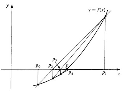
Here, we start with an initial interval [x1,x2], and we assume that the function changes sign only once in this interval. Now we find an x3 in this interval, which is given by the intersection of the x axis and the straight line passing through (x1,f(x1)) and (x2,f(x2)). It is easy to verify that x3 is given by



Now, we choose the new interval from the two choices [x1,x3] or [x3,x2] depending on in which interval the function changes sign.

The false position method differs from the bisection method only in the choice it makes for subdividing the interval at each iteration. It converges faster to the root because it is an algorithm which uses appropriate weighting of the intial end points x1 and x2 using the information about the function, or the data of the problem. In other words, finding x3 is a static procedure in the case of the bisection method since for a given x1 and x2, it gives identical x3, no matter what the function we wish to solve. On the other hand, the false position method uses the information about the function to arrive at x3.

But for a better learning here is an example, i hope you enjoy it.

Example
FInd the root of the equation X2+X-1=0, with a=0 and b=1, using the false position method.

It is easy to verify that f(x)=X2+X- 1 and f"(x)=2. Since f(1)>0 and and f"(1)>0, therefor Xo=0 and b=1.

so

For n=0 we have:


For n=1 we have:


For n=2 we have:


For n=3 we have:


For n=4 we have:


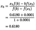
For n=5 we have:


the required root of the equation X2+X- 1=0 is =0.618.

Now i have a new topic to talk about and its Gauss-Seidel method, i find it very interesting so im going to explain it here.



After reading this, you should be able to:

1. solve a set of equations using the Gauss-Seidel method,
2. recognize the advantages and pitfalls of the Gauss-Seidel method, and
3. determine under what conditions the Gauss-Seidel method always converges.




Why do we need another method to solve a set of simultaneous linear equations?

In certain cases, such as when a system of equations is large, iterative methods of solving equations are more advantageous. Elimination methods, such as Gaussian elimination, are prone to large round-off errors for a large set of equations. Iterative methods, such as the Gauss-Seidel method, give the user control of the round-off error. Also, if the physics of the problem are well known, initial guesses needed in iterative methods can be made more judiciously leading to faster convergence.
What is the algorithm for the Gauss-Seidel method? Given a general set of equations and unknowns, we have



If the diagonal elements are non-zero, each equation is rewritten for the corresponding unknown, that is, the first equation is rewritten with on the left hand side, the second equation is rewritten with on the left hand side and so on as follows



so




As i always say, it is important to make an example so the concepts get clear, and here it is:

Example
Find the solution to the following system of equations using the Gauss-Seidel method.



Use



as the initial guess and conduct two iterations.

Solution

The coefficient matrix



is diagonally dominant an the inequality is strictly greater than for at least one row. Hence, the solution should converge using the Gauss-Seidel method.
Rewriting the equations, we get



Iteration #1



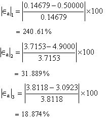
The absolute relative approximate error at the end of the first iteration is



Iteration #2



At the end of second iteration, the absolute relative approximate error is:





This is close to the exact solution vector of

A interesting iteration method that i have been searching is the Bairstow Method, which is based in the Müllers and the Newton-Raphson method.

It is very important because it allows to calculate all the polinomic roots, no matter if they are real or imaginary.



Here there are some steps that may help you to solve polynomials with this accurate method, i hope you enjoy learning this:

With a polinomyal like fn(x)you must find two factors, a cuadratic polynomial f2(x) = x2 – rx – s and fn-2(x)
.

This is the general procedure for Bairstow Method:

1.) With fn(x) and r0 and s0.

2.) With the Newton-Raphson method you calculate f2(x) = x2 – r0x – s0 and fn-2(x).

3.) You determine the roots f2(x) using the general formula.

4.) You calculate fn-2(x)= fn(x)/ f2(x)..

5.) Then you equal fn(x)= fn-2(x).

6.) If the grade of the polinomyal is greater than three, you must go back to step two.

7.) If no, you have sucesfully iterate a polynomial with Bairstows Method.

But as always we only learn making an example, so here it is.

EXAMPLE:

With the polynomial f5(x) = x5 - 3.5x4 + 2.75x3 + 2.125x2 - 3.875x + 1.25, determine the r and s values who make the equation equal to zero. Consider r0 = -1 y s0 = 2.
First iteration.

The syntethic division with the polynomial f2(x) = x2 -x + 2.0 takes as result:

f3(x) = x3 - 4.5x2 + 9.25x - 16.125 Residue = {30.75, -61.75}

Applying the Newton method we have:

-43.875.......16.75......dr.....-30.75

108.125.......-43.87.....ds.....61.75


r1 = -1.0 + 2.7636812508572213 =1.7636812508572213

s1 = 2.0 + 5.403374022767796 =7.403374022767796

Second iteration.

The syntethic division with the polynomial f2(x) = x2 -1.7636812508572213x - 7.403374022767796 giva as result:

f3(x) = x3 - 1.7363187491427787x2 + 7.091061199392814x - 1.776754563401905

Residue = {51.75640698828836, 105.68578319650365}

Applying the Newton method we have:



27.628006.......14.542693.......dr.........-51.75640

208.148405......27.62800........ds.........-105.68578


From were

r2 = 1.7636812508572213 - 0.04728019113442016 = 1.7164010597228012

s2 = 7.403374022767796 - 3.469106187802152 = 3.934267834965644
The syntethic division with the polynomial f2(x)= x2 - 1.7164010597228012x - 3.934267834965644 give as result:

f3(x) = x3 - 1.7835989402771988x2 + 3.622896723753395x + 1.3261878347051992

Residue = {12.654716254544885, 28.1881465309956}

Applying the Newton method we have:



13.83497........7.44188.........dr........-12.65471

65.679212.......13.83497........ds........-28.18814



From were

r3 = 1.7164010597228012 - 0.11666951305731528 = 1.599731546665486

s3 = 3.934267834965644 - 1.4835870659929915 = 2.4506807689726524

In brief

k..................r...............s.....................Residuo

0.................-1...............2..................30.75......-61.75

1...............1.76368.........7.403374............51.75640.....105.68578

2...............1.71640.........3.93426.............12.65471.....28.18814

3...............1.599731........2.450680............2.89958......8.1546

4...............1.33354.........2.18666.............0.760122.....2.522228

5...............1.11826.........2.113020............0.271940.....0.607688

6...............1.02705.........2.02317.............0.04313......0.11185

7...............1.00165.........2.00153.............0.00277......0.00634

8...............1.00000.........2.00000.............1.13930E-5...2.67534E-5

The solution is:

f3(x) = x3 - 2.53x2 + 2.25x - 0.625 y f2(x) = x2 - x - 2

The roots of f2(x) = x2 - x - 2, are

x1 = 2

x2 = -1

What is a truncation error?, A truncation is caused by dropping the trailing digits of a figure (number); such as by reducing 99.987 to 99.98 or 99.9. Whereas such errors may be harmless in manual computations, they can become serious mistakes in computer calculations involving thousands or millions of mathematical operations, according to that we go to be careful with the numerical approximations we do and take in account several rules for this process.

So, for avoiding this kind of error you need to considerate how to use your data before you start doing calculations, and there are two factors you may consider for this, they are called Accuracy and Precision.


Accurate means "capable of providing a correct reading or measurement." In physical science it means 'correct'. A measurement is accurate if it correctly reflects the size of the thing being measured.
Precise means "exact, as in performance, execution, or amount. "In physical science it means "repeatable, reliable, getting the same measurement each time."
We can never make a perfect measurement. The best we can do is to come as close as possible within the limitations of the measuring instruments.
Let's use a model to demonstrate the difference.
Suppose you are aiming at a target, trying to hit the bull's eye (the center of the target) with each of five darts. Here are some representative pattern of darts in the target.







Now, you can continue studying about truncation error a here is a link about a nice video about that:

http://www.youtube.com/watch?v=NByHuFBkulw

Reading i have found an interesting subject for numerical methods, and its called Roots of equation, and i am going to talk about polynomial equations. Here are three important theorems relating to the roots of a polynomial:

1.)A polynomial of n-th degree can be factored into n linear factors.
2.)A polynomial equation of degree n has exactly n roots.
3.)If (x − r) is a factor of a polynomial, then x = r is a root of the associated polynomial equation.

The cubic polynomial f(x) = 4x3 − 3x2 − 25x − 6 has degree 3.

This polynomial can be factored and written as

4x3 − 3x2 − 25x − 6 = (x − 3)(4x + 1)(x + 2)

So we see that a 3rd degree polynomial has 3 roots.

The associated polynomial equation is formed by setting the polynomial equal to zero:

f(x) = 4x3 − 3x2 − 25x − 6 = 0

In factored form, this is:

(x − 3)(4x + 1)(x + 2) = 0

We see from the expressions in brackets and using the 3rd theorem from above, that here are 3 roots, x = 3,-1/4,−2.

In this example, all 3 roots of our polynomial equation of degree 3 are real.

Since (x − 3) is a factor, then x = 3 is a root.

Since (4x + 1) is a factor, then x =-1/4 is a root.

Since (x + 2) is a factor, then x = −2 is a root.

The equation x5 − 4x4 − 7x3 + 14x2 − 44x + 120 = 0 can be factored and written as:

(x − 2)(x − 5)(x + 3)(x2 + 4) = 0

We see there are 3 real roots x = 2, 5, -3, and 2 complex roots x = ±2j, (where j = √-1).

So our 5th degree equation has 5 roots altogether.

About complex roots, the following theorem applies :

If the coefficients of the equation f(x) = 0 are real and a + bj is a complex root, then its conjugate a − bj is also a root.

So here its an example:

The factors of the polynomial x3+ 7x2 + 17x + 15 are found using LiveMath:

x3 + 7x2 + 17x + 15 = (x + 3)(x + 2 − j)(x + 2 + j)

So the roots are

x = −3

x = −2 + j and

x = −2 − j

There is one real root and the remaining 2 roots form a complex conjugate pair.

I hope you enjoyed this, and here and interesting link for you to see about newton-raphson method.

http://www.youtube.com/watch?v=lFYzdOemDj8

Many often we do numerical approximations, and we must take care of several problem who comes within, we use numerical approximation when finding an analytical solution to a differential equation is not always a practical option, numerical approximations lead to solutions that are much more readily available.

Nevertheless the are some issues related to this process, the trick to constructing a viable numerical solution of a differential is identifying a reliable approximation of the derivative.

Errors acquired during the construction of a numerical solution come from two sources: roundoff and truncation, roundoff error arises from the limited precision of computer arithmetic. The problem is compounded in that the binary representation of many fractions is irrational, enhancing the effects of the roundoff error.

The second source of error is called truncation error, this error arises when we make discrete approximations of continuous functions. This error can be, to a certain extent, limited by making the step-sizes in the discrete function as small as possible.

Now we now in what we go to be careful when we do numerical approximations, and there are few ways to minimize this errors and we will see them later on this blog.

The nodes of the following diagram represent information to be colected, sorted, evaluated and organized.



the edges of the diagram represent activities of two way communication between the nodes and the corresponding sources of information.

Reading these days about mathematical modeling i found a really interesting sort of things about it, but i asked myself, what is mathematical modeling?, and here is the answer.

Mathematical modeling is an art, because you can translate problems from an application area into tractable mathematical formulations whose theoretical and numerical analysis provides insight,answer, and guidance useful for the originating application.

Mathematical models can take many forms, including but not limited to dynamical systems, statistical models, differential equations, or game theoretic models.

But there is 1 new question, why is mathematical modeling inportant?, Mathematical modeling is indispensable in many applications, gives precision and direction for problem solution, enables a thorough understanding of the system modeled, prepares the way for better design or control of a system and allows the efficient use of modern computing capabilities. Mathematical modeling have a very importanting application in the petroleum industry and also in geosciences such as prediction of oil or ore deposits, map production and earth quake prediction inter alia.

So, now you can guess that without mathematical modelling the latest triumphs in the petroleum industry would be impossible.

And for saying good bye here is a link about another interesting subject, computer simulation.

http://www.sciencedaily.com/articles/c/computer_simulation.htm